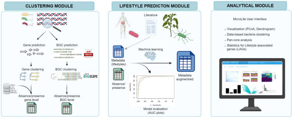
bacLIFE is a streamlined computational workflow that annotates bacterial genomes and performs large-scale comparative genomics to predict bacterial lifestyles and to pinpoint candidate genes, denominated lifestyle-associated genes (LAGs), and biosynthetic gene clusters associated with each lifestyle detected. This whole process is divided into different modules:
- Clustering module Predicts, clusters and annotates the genes of every input genome
- Lifestyle prediction Employs a machine learning model to forecast bacterial lifestyle or other specified metadata
- Analitical module (Shiny app) Results from the previous modules are embedded in a user-friendly interface for comprehensive and interactive comparative genomics.
You can find the complete wiki of bacLife here and the publication here.
If you are not familiar with using the command prompt, we recommend you to follow the introduction to Linux and R course before starting this practical course. In this course we will cover the following modules:
- Installation of Conda
- Installation of bacLIFE
- Exploring the options of bacLIFE
- Running bacLIFE with your own data
Author of this course : Pascal Nuijten
Installation of Conda
To make downloading of packages easier bacLIFE uses Conda. Conda has the following advantages for its users:
- Easily search and install thousands of data science, machine learning, and AI packages
- Manage packages and environments from a desktop application or work from the command line
- Deploy across hardware and software platforms
- Distribution installation on Windows, MacOS, or Linux
To install we open the Ubuntu terminal and download conda through the command line:
wget https://repo.anaconda.com/archive/Anaconda3-2024.10-1-Linux-x86_64.sh
Now we make the bash file executable and execute it:
				chmod +x Anaconda3-2024.10-1-Linux-x86_64.sh
./Anaconda3-2024.10-1-Linux-x86_64.sh
Now accept the terms and confirm the download location. When the execution is finished, try to execute conda in the terminal window. If it doesn’t work, the path must be exported (change USER for your computer user name!):
export PATH=/home/USER/anaconda3/bin:$PATH
Installation of bacLIFE
To download bacLIFE we open the Ubuntu terminal and move to the folder where you want to download bacLIFE. Next, we clone the bacLIFE repository using git, we advice you to download it somewhere in your windows directories:
				cd /mnt/c/Users/<your_Windows_username> #navigate to windows directory
sudo git clone https://github.com/Carrion-lab/bacLIFE.git bacLIFE
Now the next step is to move in to the folder and download the required packages. bacLIFE uses conda environments to integrate the packages that are required. The bacLIFE repository comes with .yml files to make installation of the packages easier :
				cd bacLIFE/
conda env create -f ENVS/bacLIFE_download.yml
conda env create -f ENVS/bacLIFE_environment.yml
conda env create -f ENVS/antismash.yml
conda env create -f ENVS/bigscape.yml
After installation of all the packages you now have everything requried for bacLIFE on your computer. If you want you can play around using your own genomes or genomes from the NCBI. For this course we will work with the app example. First we have to unzip the app_example.zip file in the folder. We can do this using unzip in ubuntu :
				sudo apt-get install unzip #Install unzip
unzip app_example.zip #unzip the app_example
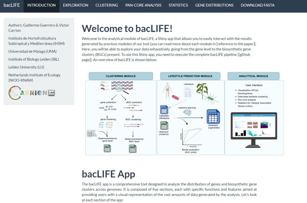
After unzipping, we can continue in R-studio. Open R-studio and browse to the bacLIFE/app_example using the right bottom file pane. Open the app.R file and press run app (in the top toolbar of the file editor in left top). R-studio prompt you to install the necessary dependencies. Next, R will launch the shiny app. The first screen will look like this:
Congratulations! You now successfully downloaded and ran bacLIFE with the example data set!
Exploring the options of bacLIFE
In this module we will go over all the tabs of bacLIFE using the example dataset. The example dataset consists of 21 genomes obtained from 5 different Pseudomonas species (fluorescens, lactis, savastanoi, syringae and sp.) annotated in 3 lifestyle groups (environmental, plant_pathogen and Unknown). The sequences and their metadata of these bacteria were uploaded and processed by BacLIFE. The toolbar of the app will give you access to all the different modules that has already been analyzed by bacLIFE:
- Introduction
- Exploration
- Clustering
- Pan-Core Analysis
- Statistics
- Gene Distributions
- Download Fasta
Introduction
In this tab you can find a brief introduction and explanation of all the modules mentioned above. Please read this page to get an idea of what the tool can do.
Exploration
This tab consists of two sub-tabs:
- Gene clusters
- Biosynthetic gene clusters
In the first one we find different input parameters (top left corner). As you can see while playing around with the settings, these parameters affect the shape of the PCoA plot in the middle of the tab. In the Database parameter we can adjust the way that the clustering is performed in the PCoA plot. We can choose different methods of plotting the data:
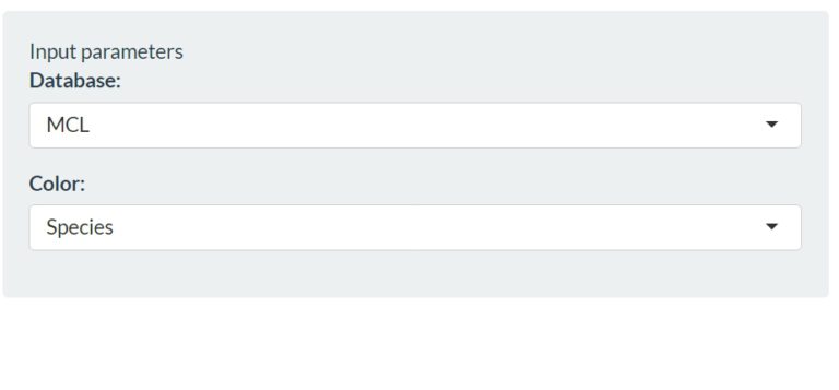
With the next input parameter we can modify the color of the dots in the Principal Coordinates Analysis (PCoA) based on the presence and absence of genes. Every dot in the PCoA represents a genome and can be colored based on their specie or based on their lifestyle. This helps to identify whether the clustering is happening based on species level or lifestyle. Since we are looking for genes that are linked to our lifestyle of interest we choose lifestyle. If we leave the default settings (MCL and Lifestyle) we obtain the following graph:
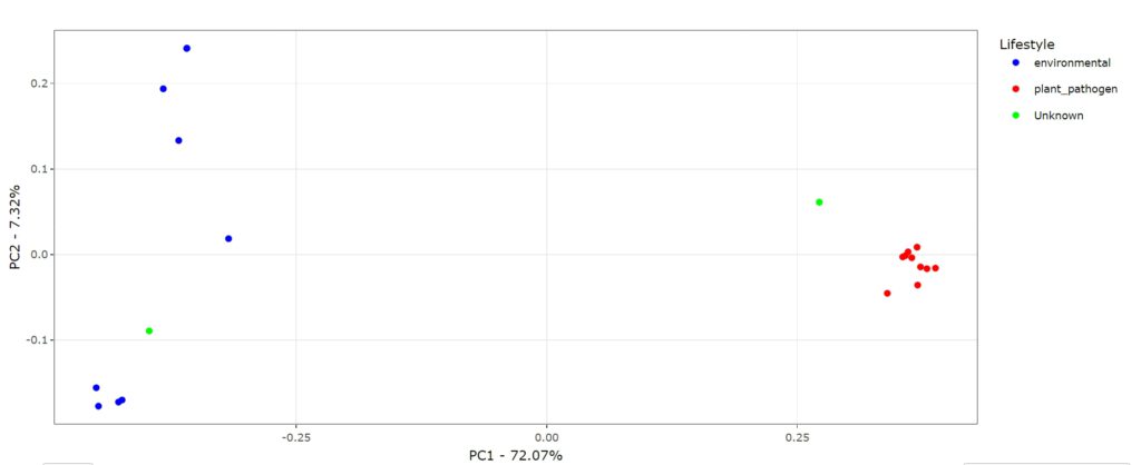
We can observe a clear differentiation between genomes associated with environmental (blue) strains and plant_pathogen (red) strains. We also have 2 unknowns strains in our graph. These are two genomes that are not annotated with either lifestyle. However, since both genomes seem to cluster together with one of the lifestyles we can predict the lifestyle associated with these unknown genomes. Below the graph you can find the data associated to the input data and below that you find the statistical test to evaluate the difference between the groups based on the input parameters. BacLIFE also offers a dendrogram function, where the clustering is visualized in a dendrogram and therefore offers you the possibility to evaluate the clustering in a different way.
Next we will look at the biosynthetic gene cluster (BGC) option. However, instead of using genes BacLIFE uses BGCs for clustering. A BGC is a cluster of multiple genes that are involved in the biosynthesis of a compound. In the first plot you can find again a PCoA but this time instead of based on the presence or absence of genes it is based on the presence or absence of BGCs. You can play around with the graphs and explore your data.
As the name of this tab is already suggesting, this whole module is made to explore your data and get an initial feeling for the genes and BGCs in your genomes.
Clustering
In this tab the actual clustering of genomes with the same lifestyle/trait is happening. To accurately predict genes related to your lifestyle/trait it is very important to have an accurate clustering. In the previous module you already got the opportunity to play around with the PCoA, now we have to tune the clustering. On the left we find a bunch of settings:
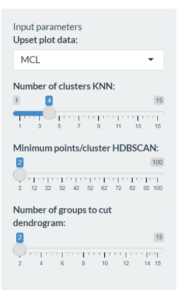
In the first column (Upset plot data:) we can choose again between the different plotting methods as in the exploration module. The next options can be used to determine the number of clusters in the different tabs: KNN clustering, HDBSCAN clustering and Dendogram clustering. The first graph in the KNN clustering tab can be useful to identify the right amount of clusters :
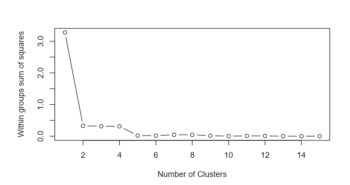
In this graph we find that the sum of squares on the y-axis and the amount of clusters on the x-axis. This means that we can find the average deviation of the data points from the mean value of a cluster. A high value correlates to a cluster with data points that are really far away from each other and a low value correlates to a cluster that contains points that are (too?) close to each other. Try to figure out what the optimal value for our example data set could be while looking at the graph? After using the graph as a first indicator for the right amount of clusters, you can start using the different tabs of this module to observe how the clustering is distributed over your samples. Try to play around with the different methods for plotting and number of clusters. If you are satisfied you can continue to the lifestyle preservation tab (right under the main toolbar). Under this tab you can find how the lifestyle/trait distribution is within your clusters:
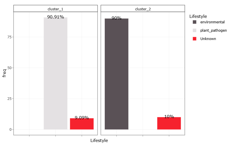
From the graph above we can observe that both clusters contain a sample with an unknown lifestyle. We can therefore predict the lifestyle of these genomes that are labeled as unknown. These kind of predictions can be very valuable for scientists that have genomes and are looking for bacteria with a certain trait/lifestyle. Think about some useful applications of these kind of predictions.
Pan-Core analysis
This tab is mainly used to study the differences between and distribution of COG annotations in the genomes. In the Pan-Genome tab you can plot different groups:
- Lifestyle –> Compare between the different lifestyles
- Species –> Compare between the different species
- Cluster_knn –> Compare between the different knn clusters
- Cluster_hdbscan –> Compare between the different hdbscan clusters
- Cluster_dendogram –> Compare between the different hdbscan clusters
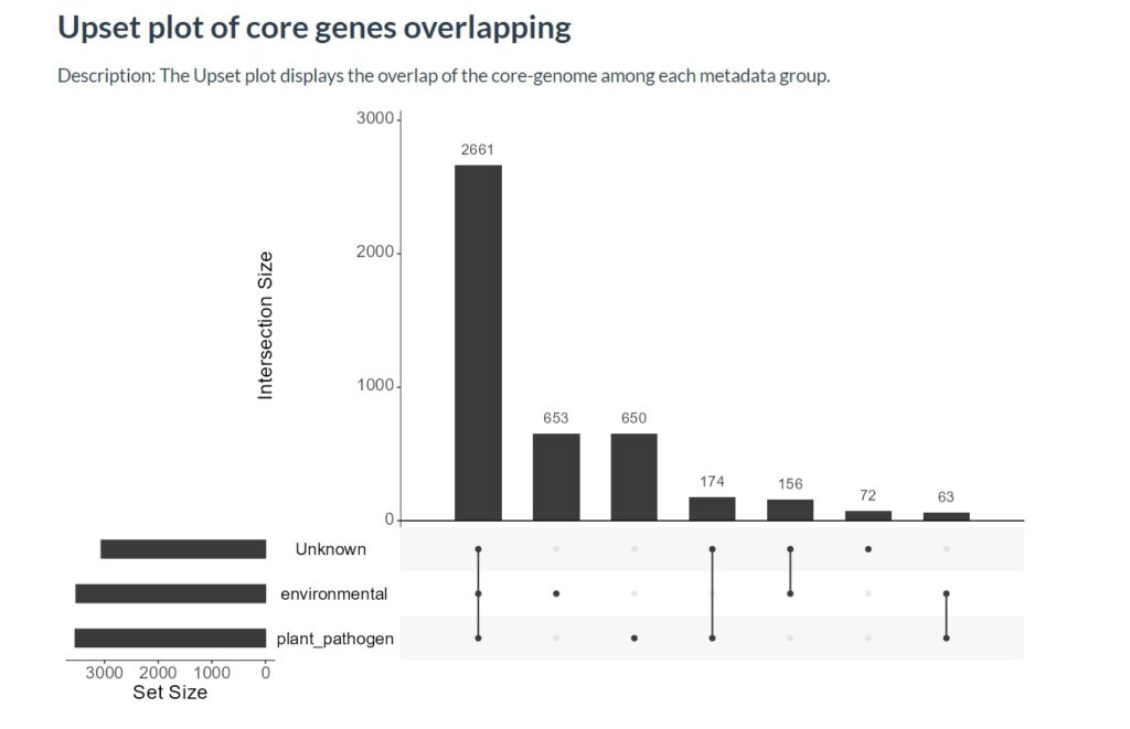
The graphs in this tab will show you bar plots that contain different COG annotations. An explanation of these COG annotations/letters can be found in the about tab. In the Core-Genome tab you can compare the distribution of the COG annotations within the full set of genomes (Graph 1), The number of core genes per cluster (Graph 2), how these core genomes are divided per group (Graph 3) and the amount of overlap/different genes per group (Graph 4). All these graphs give a great insight in how many and what kind of genes make your clusters unique. In the last tab you can search for unique genes for every genome in your dataset, this could be useful if you want to characterize what makes a specific genome cluster differently. In the following graph we can find how many of the core genes overlap per lifestyle/trait. The bar plot shows the number of genes, the dots in the bottom show in which lifestyle/trait these core genes are present.
Statistics
We consider this the most important tab of bacLIFE. After tweaking all your parameters we can use the “statistcs” module to find genes that statistically related to a lifestyle/trait. We start again with the settings on the left :
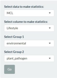
With the use of these settings and the information gained in the previous modules we can decide what kind of data(base) would be best to perform the statics on. Next we choose to use the different lifestyle for the statistics since we want to identify characteristic genes related to a certain lifestyle trait. In the last two sections we can choose the two groups used for the statistics. In this example case we will try to see the difference between environmental and plant_pathogen strains. Now we can move to the statistics tab where we can find a table containing all genes with their p-value:
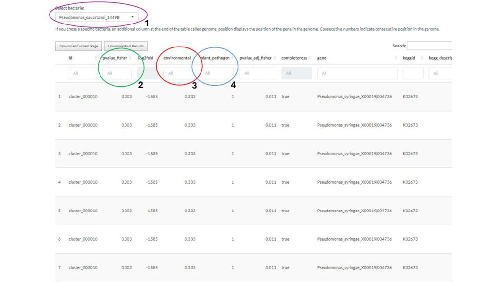
We will go over some of the important columns of this (above) graph :
- Select your bacteria: here you can filter your table to get genes from the bacteria of interest
- P-value: Filter the dataset according to the p-value (0.005?)
- Group 1 (environmental): Filter based on the percentage present in group 1
- Group 2 (plant_pathogen): Filter based on the percentage present in group 2
Gene distribution
After selecting the clusters of interest in the statistics tab (previous module), we can use the “gene distribution” tab to find how this gene cluster is distributed amongst your genomes. By selecting one of the clusters (for example : “cluster_000010”) you can easily export the cluster to your preferred format. Additionally you will obtain a graph of the presence of this gene cluster in your genomes. For the example cluster it looks like this:
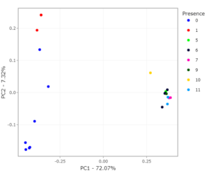
The presence of this specific example gene appears to absence/very low in the group on the left and highly abundant in the genomes on the right. If we move back to the exploration tab we can see that these clusters are related to environmental (left) and plant_pathogen (right) indicating a possible relation between cluster_000010 and the lifestyle plant_pathogen.
Download FASTA
In this last tab you can choose to download the gene cluster of interest in FASTA format. It will give you all the sequences of this cluster per genome. If the cluster appears more than once in a genome, it will give you all the different copies. This tab is especially useful for further downstream analysis of the clusters of interest. Think of a way how this data can be used in a next step?
Running bacLIFE with your own data
Now after using the bacLIFE example date you probably got excited to try it with your own data! In this part we will cover all the required steps to get your own data in bacLIFE. As bacLIFE needs a significant amount of recourses we highly recommend you to run bacLIFE in a server. As bacLIFE is a comparative genomic tool it is always advantageous to use as much data as many samples (genomes) as possible. It therefore can be good to genomes from the NCBI but its not required, if you want to run without downloading you can move to step 8.
Download genomes and reduce redundancy (optional)
Activate the conda environment to access the tools for connecting with the NCBI database and downloading genomes:
				conda activate bacLIFE_download
cd download/
2. Obtain a list of accession IDs by downloading a table from NCBI Genome Datasets.
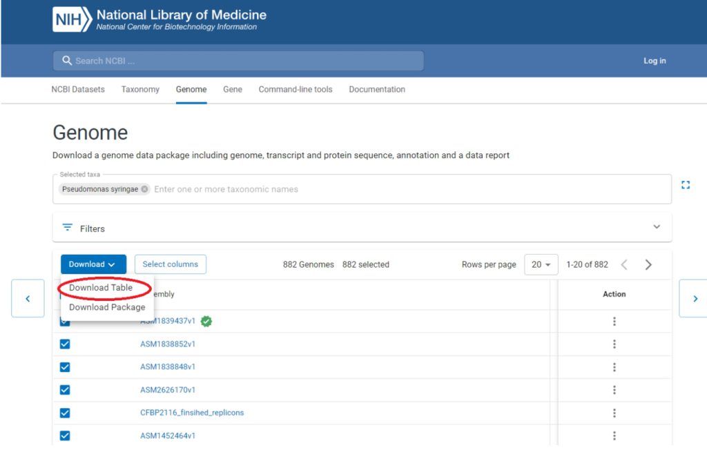
3. Convert the downloaded table to the required format (a single-column file with Assembly Accession), use this command in the download/ folder:
tail -n +2 ncbi_dataset.tsv | cut -f1 > NCBI_accs.txt
4. Download and uncompress the FASTA files. The following command will download all the genomes present in the file NCBI_accs.txt created in the previous step :
				mkdir genomes/
cd genomes/
bit-dl-ncbi-assemblies -w ../NCBI_accs.txt -f fasta -j 10
gzip -d ./*.gz
5. Download metadata and remove redundancy at >99% Average Nucleotide Identity (ANI). This step downloads metadata for each genome to enable accurate name annotation. Next, the genomes are clustered based on 99% Average Nucleotide Identity (ANI) to eliminate redundancy among nearly identical genomes.
				cd ../
python main_script_download.py
6. Now we will make sure everything is ready :
- “genomes_renamed/”: Directory where the non-redundant genomes with the filenames ready for bacLIFE are stored.
- “METADATA_MERGED.txt”: File with the following columns: ‘scientific_name’, ‘NCBIid’, ‘cluster_membership’, ‘representative’ and ‘bacLIFE_name’
7. Deactivatethe conda environment bacLIFE_download:
conda deactivate bacLIFE_download
8. Activate bacLIFE clustering module conda environment and download dependencies.
				conda activate antismash_bacLIFE
download-antismash-databases
conda deactivate

conda activate bacLIFE_environment
python src/download_dependencies.py
9. To prepare the input files they must be FASTA assemblies stored in the data/ directory, all with name that should follow the format “Genus_species_strain_O.fna“. You have some example genomes in correct name format in the data/ directory. Remember to remove them so they are not incorporated in your analysis
rm data/*
9. If genomes were downloaded as described in the previous section ‘Download genomes and reduce redundancy’, the folder directory download/genomes_renamed/ already contains the genome files in the correct name format and they only have to be moved to the data/ folder .
mv download/genomes_renamed/* data/
10. Once you have your genomes in the format “Genus_species_strain_O.fna“* and stored in the data/, you must use the script src/rename_genomes.R to change the input genome strain names into a bacLIFE friendly format in the following way:
Rscript src/rename_genomes.R data/ names_equivalence.txt
11. This script changes the name of the input genome files by replacing the strain name into a barcode to avoid bacLIFE crashes
I.e Pseudomonas_fluorescens_FDAARGOS-1088_O.fna –> Pseudomonas_fluorescens_X0001_O.fna
The file “names_equivalence.txt” contains the correspondent name matching and needs to be present in the main directory before running bacLIFE.
*In the genome format name, the user must avoid adding any special characters, that is not a alphabet letter, number , dash or dot. This applies specially to the strain name which also should be of less than 10 characters long.
After running the renaming script is good to do a quick check of the genome names and the names_equivalence file. Sometimes, weird characters or names can results in a genome missing from the equivalence file or having an incomplete name.
12. The configuration file ‘config.json’ allow users to change some important parameters that are used during the workflow:
				{
    "threads" : 24,
    "mcl_inflation_value": 3.0,
    "linclust_identity": 0.95,
    "threads_prokka_antismash": 8,
    "phylo_database" : "amphora2"
}
- ‘threads’: number of cpus or threads to use.
- ‘mcl_inflation_value’: The inflation value utilized in the Markov clustering process determines the level of granularity in the resulting clusters. A default value of 3.0 is employed.
- ‘linclust_identity’: The default sequence similarity threshold applied for clustering prior to the Markov clustering is set at 0.95, which corresponds to a 95% sequence similarity level.
- ‘threads_prokka_antismash’: number of cpus or threads to use for prokka and antismash
- ‘phylo_database’: Specifies the marker database to be used in PhyloPhlan3, with the default setting being “amphora2”.
-j specifies the number of maximum CPU cores to use for the whole process. If this flag is ommitted, Snakemake will use all the available CPU cores in the machine. Make sure this number is never lower then threads or “threads_prokka_antismash” in the “config.json”.)
snakemake -j 24 --use-conda
mapping_file.txt file. This file is generated at the end of the clustering module in the main folder. It consists of a two column tab-separated file where the first column specifies the genome name (as established in the data/ directory) and the second column specifies the Lifestyle of that genome. Every genome lifestyle is annotated as ‘Unknown’ when the file is generated. User have to manually annotate the genomes with their information of interest. Genomes with no lifestyle information must be annotated as “Unknown”. Note that additional columns can be added to the file with other metadata information.src/classifier.R and specifying the location of mapping_file.txt and MEGAMATRIX_renamed.txt in addition to the column name of the metadata variable that the user wants to predict
Rscript classifier_src/classifier.R mapping_file.txt MEGAMATRIX_renamed.txt Lifestyle
ROC plots showing the model evaluation for the different classes present in the metadata column shosen are generated and stored in classifier/
If good accuracy is accomplished, the user can use the model for predictions of genomes labeled as ‘Unknown’ in the mapping file. The resulting augmented metadata is stored in the new file mapping_file_augmented.txt
16. In order to initiate the shiny app, the following snakemake output files need to be droped in the ‘Shiny_app/input/’ directory.
MEGAMATRIX_renamed.txtmapping_file.txtormapping_file_augmented.txt(ifmapping_file_augmented.txtis used, name should be changed tomapping_file.txtin the ‘Shiny_app/input/’ so it can be readed in the app)intermediate_files/BiG-SCAPE/big_scape_binary_table_renamed.txtintermediate_files/BiG-SCAPE/annotation.txtintermediate_files/combined_proteins/combined_proteins.fastanames_equivalence.txt
To be able to see the antismash user interface of each input genome within the bacLIFE Shiny app, the folder intermediate_files/antismash/ needs to be placed in the Shiny_app/ folder.
Users have the option to either manually relocate these files or utilize the following script from the main bacLIFE directory to automatically transfer all the required files to the ‘Shiny_app/input/’ directory.
python src/prepare_app_inputs.py
After having prepared these input files, users should move the working directory to Shiny_app/ and open the script app.R in Rstudio and click in the upper right ‘run app‘ button to initiate the bacLIFE app and enjoy visualizing all their results! Note that user may move the Shiny_app/ folder and all its content to a local computer and lunch Rstudio locally. All packages needed for the app are automatically installed when running the app if they are not installed. / An example of the app can be found in app_example.zip
The bacLIFE app is a comprehensive tool designed to analyze the distribution of genes and biosynthetic gene clusters across genomes. It is composed of five sections, each with specific functions and features aimed at providing users with a visual representation of the vast amounts of data generated by the analysis.